the author

Scheimpflug's rule : a simple ray-tracing for high school ?

(Version Française)

Emmanuel BIGLER

Résumé : We show here how Scheimpflug's rule can be found by an elementary ray tracing procedure based on common rules of image formation in a thin positive lens.

Introduction

Photographic textbooks on Large Format cameras present most of the times Scheimpflug's rule without any proof, even if elementary ray tracing procedures for image formation by a positive lens (position, magnification) are always presented and sometimes illustrated in detail.

A good reason is that anybody attempting to re-start from Mr. Scheimpflug's complex original patent [1] would have hard times to use this well-know large format photographic rule in practice.

Elegant proofs exist (see Bob Wheeler's documents [2] as well as Q.-Tuan Luong's web site [3]) however they require a substantial knowledge of high-level geometry and mathematics. Considering the minimum knowledge of geometrical optics taught in high school in France up to the '60s, I realized that a student of such a high school, following basic rules of image formation and ray tracing, could easily find how the image of a slanted object is in fact located in another slanted direction obeying Scheimpflug's rule, i.e. the 2 planes intersecting in the lens plane. So let us, for few minutes, go back to school and apply the basic rules of geometrical optics.

Scheimpflug's rule as a consequence of a simple ray tracing

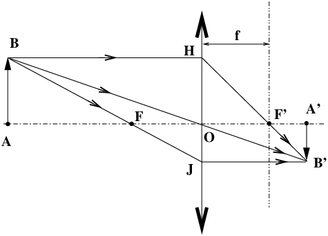
In elementary courses, one of the first ray tracing procedures that students learn is how to find the image A'B' of an object AB through a thin positive lens of focal distance f. As a starting point this object is always taken perpendicular to the optical axis. The following rules apply (see figure 1), they are nothing more than what is usually taught in elementary classes.

1. any incident ray, parallel to the optical axis e.g. BH crosses on exit the optical axis in the image focal point F', following the path HF'B',
   
   

2. any incident ray crossing the lens through its optical center, e.g. BO, is not deflected on output and follows the path OB',
   
   

3. all rays emitted by a single (object) light point A cross each other in the image A', same for B and B',
   
   

4. if AB is an object perpendicular to the optical axis, its image A'B' is also perpendicular to the axis.

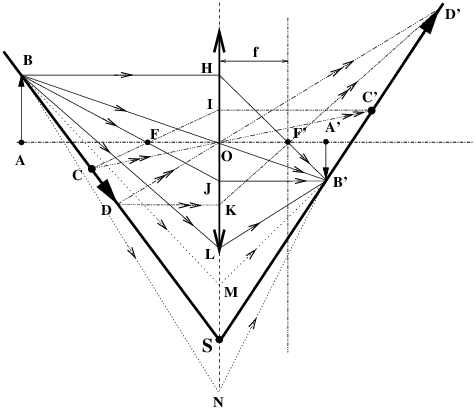
Surprisingly, professors hardly ever ask the students to find where the image of a slanted object like CD is located. It is not so difficult, however, simply following the above mentioned rules, to find CIC' (rule #1) and COC' (rule #2), then DKD' et DOD'; nothing spectacular or difficult here, however the relationship that may exist between the planes BCD et B'C'D' is still totally unclear.

One should in fact keep in mind an additional rule, always presented by professors


rule #5 : in all ray-tracing of geometrical optics, one may expand the vertical scale by any factor without changing anything to the previous rules, as if the lens was unlimited in the direction perpendicular to its axis.


Thus, a well-disciplined student will plot without any question the following rays: BLB', then BMB' and BSB' and even BNB' in total compliance with all the above mentioned rules, since all rays emitted by the object B must intersect in the image point B'.

Now this is just what we need to say:


Let us forget (rule #5) that the lens is actually limited, and let us consider a ray like BCDS; this ray must go through all successive images B', C' and D' of light sources B, C, and D according to rule #3, with the special case of S being identical to its image.


The conclusion is that the image of the slanted object plane BCDS is the slanted image plane SB'C'D', in other words nothing but Scheimpflug's rule[1].

Final remarks

• A first difficulty arises from the fact that, in practice, the f-stop actually limits the usable part of the lens to such a small diameter that it may seem absurd to consider an ``imaginary'' ray like BCDSB'. But when, in practice, starting from a very small aperture (rays in the vicinity of BOB') the f-stop is gradually opened to allow other rays like BLB' to enter the lens, one does nothing else but obey all basic rules, those rules being still valid even if we extrapolate according to rule #5 up to the ``imaginary'' ray BCDSB'.
  
  

• A second difficulty comes from the fact that a photographic lens is never a single element but a ``thick'' compound optical system. In fact, to get a good idea of what happens in a real lens, one should simply take a pair of scissors and cut fig.2 along the lens plane HON and separate both sides parallel to the optical axis by a distance HH' (positive for a wide-angle ``retrofocus'' lens or even negative for a telephoto) equal to the distance between principal planes HH' of the system (or nodal planes, they are identical in air). The ``optical thickness`` HH' of a photographic lens is in the range of a few centimeters. In practical terms hardly anything will change with respect to what has been derived for a single thin lens element. Simply the planes BCDS and SB'C'D' will intersect somewhere between the principal planes H and H'.

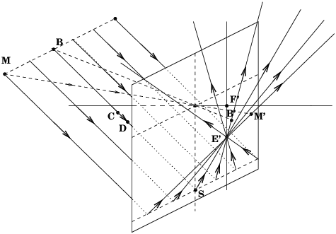
• A last difficulty is that we have only considered in this derivation rays propagating in a plane containing the optical axis (technically : meridian rays) but what about a whole 3-D object plane? Then again, ray tracing (fig.3) will solve the problem. Consider a family of parallel rays propagating along a rectangular grid plotted in the slanted object plane, all those rays being parallel to the ray BCDS. According to another well-know rule, namely that parallel rays on input will all cross on output as a single point E' located in the focal plane, we can easily see that after refraction by the lens, the locus of all emerging Scheimpflug's rays coming from those parallel incident rays is actually another slanted plane in 3-D space, this plane intersecting with the plane of fig.2 as the meridian ray SB'. As a by-product we can see also that a rectangular grid will be distorted and rendered as a bunch of converging rays, the original rectangles being distorted as a trapezoidal shapes.

Références

[1]	British patent by Theodor Scheimpflug, 1904, http://www.trenholm.org/hmmerk/TSBP.pdf
[2]	Bob Wheeler, "Notes on view camera", http://www.bobwheeler.com/photo/ViewCam.pdf
[3]	Q.-Tuan Luong, http://www.largeformatphotography.info/scheimpflug.jpeg

Emmanuel Bigler 16 novembre 2002

dernière modification de cet article : 2002